4

Is there a way to calculate bandwidth of an classical dipole antenna having this information:

  • center frequency
  • wire velocity
  • wire diameter

I would disregard antenna height, to simplify.

I am not targeting high precision calculation, just rough but usable. I need this to be calculated, not measured.

Pedja YT9TP
  • 890
  • 6
  • 13

3 Answers3

5

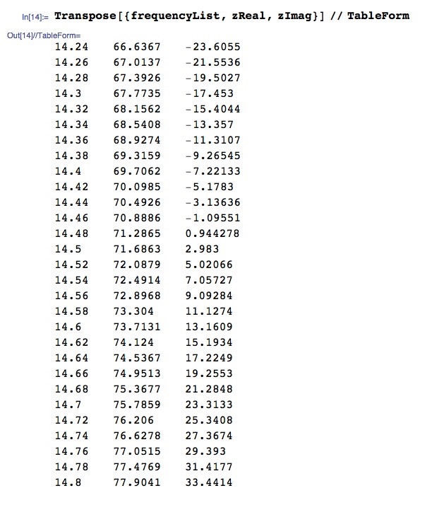
Assuming the antenna is in free space, you only need to know the length and diameter of the wire used to construct the dipole. The math is hairy but I wrote a program to do the calculations. Here is the SWR (assuming a 50 ohm source) and feedpoint impedance for a dipole 10 meters long, with a diameter of 2.053mm:

14.100 MHz: SWR 2.07,  61.3 + j-39.6
14.130 MHz: SWR 1.98,  61.7 + j-36.8
14.160 MHz: SWR 1.89,  62.0 + j-34.0
14.190 MHz: SWR 1.81,  62.4 + j-31.3
14.220 MHz: SWR 1.73,  62.8 + j-28.5
14.250 MHz: SWR 1.66,  63.2 + j-25.7
14.280 MHz: SWR 1.60,  63.5 + j-23.0
14.310 MHz: SWR 1.54,  63.9 + j-20.2
14.340 MHz: SWR 1.48,  64.3 + j-17.4
14.370 MHz: SWR 1.44,  64.7 + j-14.7
14.400 MHz: SWR 1.40,  65.1 + j-11.9
14.430 MHz: SWR 1.37,  65.5 + j-9.1
14.460 MHz: SWR 1.35,  65.8 + j-6.4
14.490 MHz: SWR 1.33,  66.2 + j-3.6
14.520 MHz: SWR 1.33,  66.6 + j-0.9
14.550 MHz: SWR 1.34,  67.0 + j 1.9
14.580 MHz: SWR 1.36,  67.4 + j 4.7
14.610 MHz: SWR 1.39,  67.8 + j 7.4
14.640 MHz: SWR 1.43,  68.2 + j10.2
14.670 MHz: SWR 1.47,  68.6 + j13.0
14.700 MHz: SWR 1.52,  69.0 + j15.7
14.730 MHz: SWR 1.57,  69.4 + j18.5
14.760 MHz: SWR 1.63,  69.9 + j21.3
14.790 MHz: SWR 1.69,  70.3 + j24.1
14.820 MHz: SWR 1.75,  70.7 + j26.8
14.850 MHz: SWR 1.82,  71.1 + j29.6
14.880 MHz: SWR 1.89,  71.5 + j32.4
14.910 MHz: SWR 1.97,  71.9 + j35.1
14.940 MHz: SWR 2.05,  72.4 + j37.9

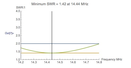
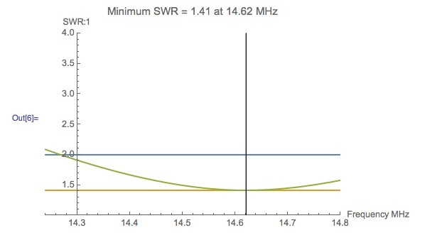
To calculate the bandwidth we must define what we mean by bandwidth. Let's define it as the range through which SWR is 2:1 or less. In that case, this antenna works from about 14.125 to 14.920 MHz, for a bandwidth of 795 kHz.

We can express that as a fractional bandwidth:

$$ {14.125 - 14.920 \over (14.125 + 14.920) / 2} = 5.5\% $$

You'll find that similar dipoles will have a similar fractional bandwidth. For example if I run the numbers for the same wire diameter but now 20 meters long, I find a fractional bandwidth of 5.0%.

This decrease in bandwidth is due to the wire diameter being thinner relative to wavelength. A thicker dipole relative to wavelength will have more bandwidth than a thinner one. The bandwidth is actually quite sensitive to the conductor radius.*

For example, if I make a dipole for the 2 meter band from 3/4 copper pipe, the fractional bandwidth goes up to 15% on account of the much smaller wavelength and the much thicker wire.

If you need just a rough calculation, then an estimate of fractional bandwidth is sufficient. Just multiply the center frequency by the fractional bandwidth.

Here's the source for the program, if you want to do your own calculations:

#!/usr/bin/python3

from math import sin, cos, log
from scipy.special import sici
from scipy.constants import pi, c

def sin2(t):
    return sin(t)**2

def ci(t):
    '''cosine integral'''
    return sici(t)[1]

def si(t):
    '''sine integral'''
    return sici(t)[0]

# euler constant
gamma = 0.577215664901532

# impedance of free space
Z0 = 376.73031

def R(f, L, a):
    k = 2*pi*f/c

    return Z0 / (2*pi*sin2(k*L/2)) * (
        gamma
        + log(k*L)
        - ci(k*L)
        + .5 * sin(k*L) * (
            si(2*k*L)
            -2*si(k*L)
        )
        + .5 * cos(k*L) * (
            gamma
            + log(k*L/2)
            + ci(2*k*L)
            - 2*ci(k*L)
        )
    )


def X(f, L, a):
    k = 2*pi*f/c

    return Z0 / (4*pi*sin2(k*L/2)) * (
        2*si(k*L)
        + cos(k*L) * (
            2*si(k*L)
            - si(2*k*L)
        )
        -sin(k*L) * (
            2*ci(k*L)
            - ci(2*k*L)
            - ci(2*k*a**2/L)
        )
    )


def Z(f, L, a):
    return complex(R(f, L, a), X(f, L, a))


def SWR(Z_l, Z_s):
    reflection_coef = (Z_l - Z_s) / (Z_l + Z_s)
    return (1 + abs(reflection_coef)) / (1 - abs(reflection_coef))


# in Hz
f_lower = 137e6
f_upper = 155e6
step = 750e3

# in meters
length = 0.942
diameter = 19.05e-3

# in ohms
source = complex(50)

f = f_lower
while f < f_upper:
    load = Z(f, length, diameter)
    print('    %6.3f MHz: SWR %4.2f, %5.1f + j%4.1f' % (f/1e6, SWR(load, source), load.real, load.imag))
    f += step

* Note how $a$ appears only in the $\mathrm{Ci}(2ka^2/L)$ term, and the cosine integral function asymptotically approaches $-\infty$ at 0.

Phil Frost - W8II
  • 52,635
  • 8
  • 91
  • 225
1

I have used NEC4 to model the antenna parameters used by Phil Frost in his answers. I am doing this primarily for my own curiosity to see how close or far apart his answers from his algorithm are from the NEC4 modeling of the same antenna.

The antenna being modeled is a center fed dipole, 10-meters total length, with #12 copper wire. The only difference between the previous answer and mine is that Phil Frost used 3 mm for the diameter of the #12 wire and I am using 2.053 mm which is a value I get from this web-site: American Wire Gauge.

My first run is for a FREE-SPACE solution and the only thing I am showing at this time is the computed SWR plot.

20 meter dipole SWR

The plot is generated from Mathematica using the following procedure:

  1. Run NEC4 on input data to produce solution output file.
  2. Scrape output file to produce curated data file.
  3. In Mathematica, read curated data file.
  4. In Mathematica, create Interpolation Function on data to compute SWR.
  5. Plot function.

The data used is the antenna input impedance calculated by NEC4 versus a standard 50-ohm RG-8X coaxial cable made by CableXperts (using their data). The actual data computed is shown in the table below. The three columns left to right are frequency, real value of impedance, imaginary value of impedance.

enter image description here

The above plot shows the SWR minimum of 1.42 at 14.44 MHz. The minimum is marked by the yellowish-orange horizontal line. On my SWR plots I always mark the SWR 2:1 horizontal line as the bandwidth that I am interested in is between the intersection points of the SWR curve and the 2:1 SWR horizontal line. Other people may use other SWRs to determine bandwidth (such as 3:1).

The resonant frequency of the antenna is when the impedance is a pure resistance. This occurs when the reactance, the imaginary value, is zero. The following plot shows where the reactance crosses the zero value at approximate frequency of 14.475 MHz.

enter image description here

The frequencies below the resonant frequency have negative reactance values meaning that these are capacitive reactance. Capacitive reactance indicates that the antenna is too short for those longer wavelengths. Given that the resonant frequency of 14.475 MHz is outside of the 20-meter amateur band, a better antenna solution would demand a longer antenna than the 10 meters as modeled.

The following plot shows the SWR of the same physical antenna but this time it is modeled over a real ground profile using a Sommerfeld/Asymptotic solution implemented by NEC4. The elevation of the antenna over ground is 10 meters. The key ground parameters are conductivity of 0.004 siemens/meter and a relativity permittivity of 12.

Notice that the minimum SWR is now slightly lower than before and the frequency where minimum SWR occurs has shifted slightly to a higher value.

enter image description here

K7PEH
  • 3,028
  • 13
  • 14
-3

Bandwidth of an antenna is the frequency range which the antenna can operate correctly. The antenna's bandwidth is the range in Hz that the antenna will exhibit an SWR < 2:1.

Bandwidth can also be described as the percentage of the center frequency of the band:

BW=100*((FH−FL)/FC)

(FH is the highest frequency in the band, FL is the lowest frequency in the band, and FC is the center frequency in the band.)